Lecture 10 Stock market monte-carlo simulation

10.1 Case study, growth of portfolio

Case-1: Reproduce the following columns from 4 to 7 using R codes.

r	R = (1+r)	t	Year1	Year2	Year3	Year4	Cumulative
(1)	(2)	(3)	(4)	(5)	(6)	(7)	(8)
\(-0.05\)	\(0.95\)	\(1\)	\(0.95\)	\(0\)	\(0\)	\(0\)	\(0.95\)
\(0.1\)	\(1.1\)	\(2\)	\(0.95 \times 1.1 = 1.045\)	\(1.1\)	\(0\)	\(0\)	\(2.145\)
\(0.2\)	\(1.2\)	\(3\)	\(0.95 \times 1.1 \times 1.2 = 1.254\)	\(1.1 \times 1.2 = 1.32\)	\(1.1\)	\(0\)	\(3.674\)
\(0.3\)	\(1.3\)	\(4\)	\(0.95 \times 1.1 \times 1.2 \times 1.3 = 1.643\)	\(1.1 \times 1.2 \times 1.3 = 1.716\)	\(1.2 \times 1.3 = 1.56\)	\(1.3\)	\(6.219\)

Lets do it in very inefficient way first to develop intuition.

# This one is column (1)
r <- c(-0.05, 0.1, 0.2, 0.3)
# This is column (2)
R <- 1 + r

# To find the column (4)
c4 <- cumprod(R)
c4
#> [1] 0.9500 1.0450 1.2540 1.6302

# To find the column (5), we have to think slightly carefully.
r <- c(0.1, 0.2, 0.3)
R <- 1 + r
cumprod(R)
#> [1] 1.100 1.320 1.716
c5 <- c(0, cumprod(R))
c5
#> [1] 0.000 1.100 1.320 1.716

# To find the column (6), we have to think slightly carefully.
r <- c(0.2, 0.3)
R <- 1 + r
c6 <- c(0,0,cumprod(R))

# To find the column (7), we have to think slightly carefully.
r <- c(0.3)
R <- 1 + r
c7 <- c(0,0,0,cumprod(R))

my_table <- cbind(c4,c5,c6,c7)

my_table
#>          c4    c5   c6  c7
#> [1,] 0.9500 0.000 0.00 0.0
#> [2,] 1.0450 1.100 0.00 0.0
#> [3,] 1.2540 1.320 1.20 0.0
#> [4,] 1.6302 1.716 1.56 1.3

# Lets rowwise sum with rowSums. Note that "S" is capital letter 
my_table <- cbind(my_table, rowSums(my_table))

my_table
#>          c4    c5   c6  c7       
#> [1,] 0.9500 0.000 0.00 0.0 0.9500
#> [2,] 1.0450 1.100 0.00 0.0 2.1450
#> [3,] 1.2540 1.320 1.20 0.0 3.7740
#> [4,] 1.6302 1.716 1.56 1.3 6.2062

We are using two new functions cbind() and rowSums(). Let me discuss that. The cbind() function combines vectors, matrices, or data frames by columns in R. This function takes the objects to be combined as arguments and returns a new object containing the combined data. Like cbind(), we also have rbind() to combine vectors, matrices, or data frames by rows.

In R, the rowSums() function is used to compute the sum of the values in each row of a matrix or data frame. This function takes as its first argument the matrix or data frame to be summed and returns a vector containing the row sums. Similar to colSums() to compute the sum of the values in each column of a matrix or data frame

The above example is very manual. So let’s do this using for loop.

r <- c(-0.05, 0.1, 0.2, 0.3)
R <- 1+r
# Initialize a list() rather than an atomic vector
portfolio <- list()
for(i in 1:length(R)){
  # Here is the zero vector
  zero_vector <- rep(0,i-1)
  # Here is the vector of cumulative product.
  cumprod_vector <- cumprod(R[i:length(R)])
  
  # We concatenate the zero and cumulative product vector
  my_result <- c(zero_vector, cumprod_vector)
  
  # Let's put this results into a list.
  portfolio[[i]] <- my_result
}

# Print the value of portfolio
portfolio
#> [[1]]
#> [1] 0.9500 1.0450 1.2540 1.6302
#> 
#> [[2]]
#> [1] 0.000 1.100 1.320 1.716
#> 
#> [[3]]
#> [1] 0.00 0.00 1.20 1.56
#> 
#> [[4]]
#> [1] 0.0 0.0 0.0 1.3

We still need to do some more work. We need to column-wise bind the results from the list. For this, we will use a very powerful function called do.call(). In R, the do.call() function is used to evaluate a function call with arguments given in a list or a data frame. This function takes as its first argument the name of the function to be called and as its second argument, the list or data frame containing the arguments to be passed to the function. Within do.call(), we will use cbind().

my_table <- do.call(cbind, portfolio)

Lets take the rowSums() and plot the growth of the portfolio.

portfolio_value <- rowSums(my_table)
plot(portfolio_value, type = "b", col = "red", lwd = 2)

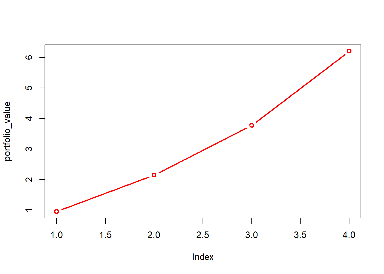
Case-1: Plot how your 1 dollar recursively invested portfolio grows using the S&P 500 Index Stock Market growth.

10.2 Case, Monte Carlo simulation of stock market

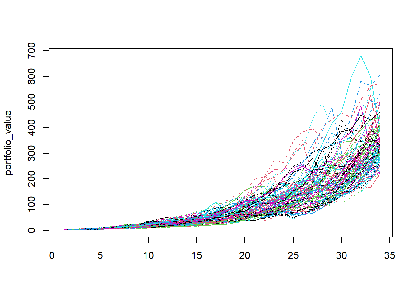
Case-2: What the past 35 years looked like, it might look different in the upcoming future. You decided to remain invested for the next 35 years. You don’t know the future sequences of growth or risk. So you can simply randomize the historical sequences as these returns could occur in any random order. Simulate in 1000 trials R. Show the evolution of the cumulative portfolio value over 35 years.

snp_ret <- c(...)
portfolio_value <- ...
for(...){
  r <- sample(...)
  R <- ...
  portfolio <- ...
  for(i in 1:length(R)){
    zero_vector <- ...
    cumprod_vector <- ...
    portfolio[[i]] <- ...
  }
  portfolio_value[[j]] <- rowSums(do.call(..., ...))
}
portfolio_value <- ...(..., ...)

matplot(portfolio_value, type = "l")

matplot(portfolio_value, type = "l")