Lecture 11 Confidence interval, z-scores, hypothesis testing
11.1 Confidence interval
11.1.1 Previous example on the day trading.
Let’s imagine I decided to day trade (hashtag, not financial advice). My trading philosophy is straightforward. I put stop loss at 100 dollars and took profit at 125 dollars. Or if my stock goes down, I limit the loss to 100 dollars, and if my stock goes up, I limit the win to 125. However, call it your skill or the way Mr. Market works. I am no better than a coin flip, so it’s 50% likely that I make or lose. I can trigger trade about 99 times a day, and the trading software limits me. However, I can come back tomorrow and trade again. We have 200 trading days in a year, and I have been doing this for the past five years. What are my cumulative portfolio values at 90%, 95%, and 99% confidence intervals? What is the probability that I will suffer loss? For the sake of simplicity, there are no fees or commissions.
sum_total_winnings <- c()
for (j in 1:10000) {
  total_winnings <- c()
  for (i in 1:50) {
    total_winnings[i] <- sample(x = c(125,-100),
                                size = 1,
                                replace = T)
  }
  sum_total_winnings[j] <- sum(total_winnings)
}
This code simulates the game where a player can win or lose money. It uses a for loop to simulate the game being played 1000 times, and it calculates the total winnings for each game.
The code begins by defining an empty vector called sum_total_winnings. This vector will be used to store the total winnings for each game.
Next, the code uses a for loop to simulate the game being played 1000 times. The code defines an empty vector called total_winnings for each iteration of the loop. This vector will store the winnings for each round of the game.
The code then uses another for loop to simulate 50 rounds of the game. For each round, the code uses the sample() function to randomly select either a win of $125 or a loss of $100. The result is stored in the total_winnings vector.
Once all 50 rounds of the game have been simulated, the code calculates the sum of the winnings in the total_winnings vector using the sum() function. This gives the total winnings for the current game. The code then stores this value in the sum_total_winnings vector.
After all, 1000 games have been simulated, and the total winnings for each game have been calculated, the code will have a vector called sum_total_winnings that contains the total winnings for each game.
You can use the hist() function in R to plot a histogram of the sum_total_winnings vector. Here is an example of how you could do this:
# Plot a histogram of the sum_total_winnings vector
hist(sum_total_winnings)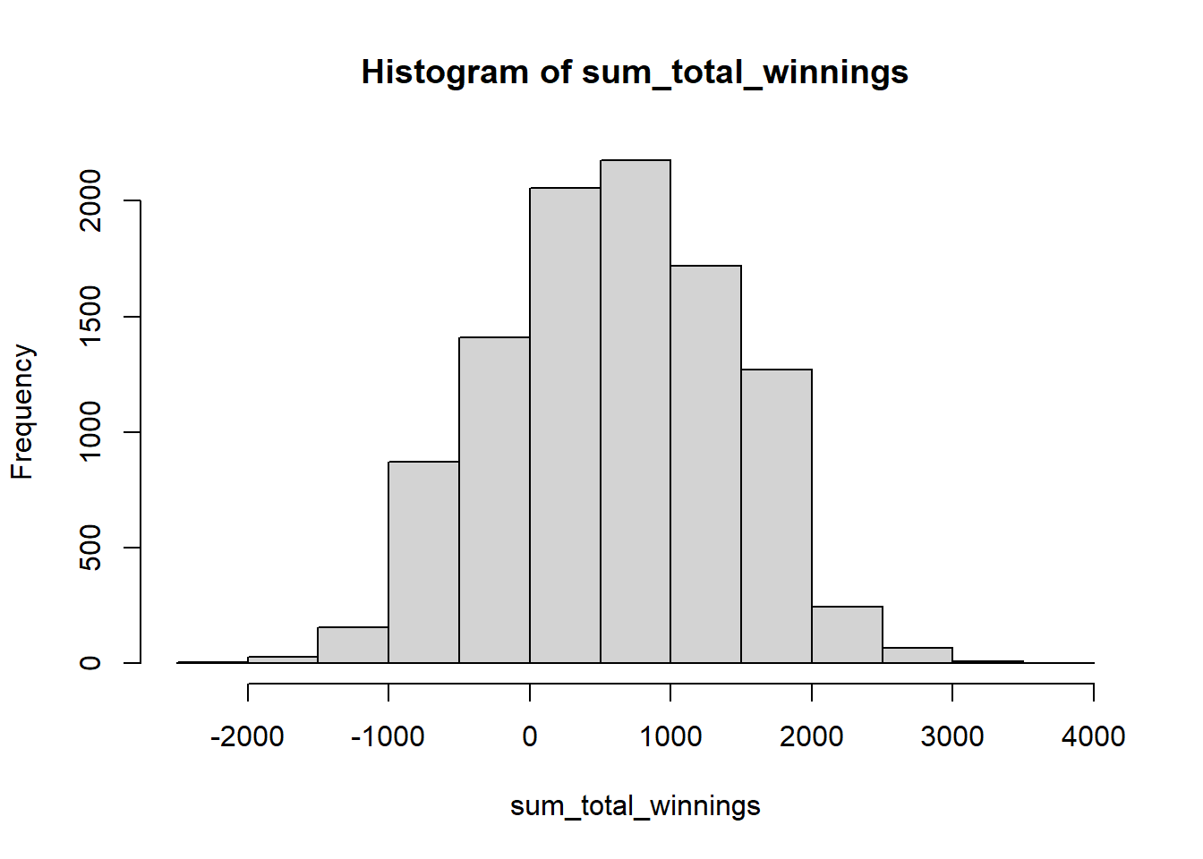
This code will generate a histogram of the values in the sum_total_winnings vector. The histogram will show the frequency of each value in the vector, allowing you to see how often each total winnings amount occurred in the simulated games.
You can customize the appearance of the histogram using various arguments to the hist() function.
Looking at the histogram, we can quickly make educated guesses for min, max, and mean. For example, to find the minimum, maximum, and mean of the sum_total_winnings vector, you can use the following R code:
# Find the minimum value in the sum_total_winnings vector
min(sum_total_winnings)
#> [1] -2075

# Find the maximum value in the sum_total_winnings vector
max(sum_total_winnings)
#> [1] 3550

# Find the mean of the sum_total_winnings vector
mean(sum_total_winnings)
#> [1] 610.6225
Looking at the histogram and the mean statistics, it is likely that this game generates an average winning of 610.6225, which is not so bad.
But how confident are we about this average estimate of winnings? Well, to be 95% sure or confident, the average will be in between the 2.5% and 97.5% quantiles. To find the 2.5% and 97.5% quantiles of a vector in R, you can use the quantile() function. Here is an example of how you could use this function to find the 2.5% and 97.5% quantiles of the sum_total_winnings vector:
# Find the 2.5% and 97.5% quantiles of the sum_total_winnings vector
quantiles_value <- quantile(sum_total_winnings, probs = c(0.025, 0.975))
The 2.5% quantile is the value below which 2.5% of the values in the sum_total_winnings vector fall. Similarly, the 97.5% quantile is the value below which 97.5% of the values in the sum_total_winnings vector fall. In other words, the 95% confidence interval is the range of values between the 2.5% and 97.5% quantiles. Thus it suggests we are 95% confident that the average winning ranges between -950 and 2200.
To add a 95% confidence interval and mean to a histogram of the sum_total_winnings vector, you can use the abline() function in R. Here is an example of how you could do this:
# Plot a histogram of the sum_total_winnings vector
hist(sum_total_winnings)

# Calculate the 2.5% and 97.5% quantiles of the sum_total_winnings vector
quantiles <- quantile(sum_total_winnings, probs = c(0.025, 0.975))

# Calculate the mean of the sum_total_winnings vector
mean_value <- mean(sum_total_winnings)

# Add lines to the histogram showing the 95% confidence interval and the mean
abline(v = quantiles, col = "red", lty = 9)
abline(v = mean_value, col = "blue", lty = 2)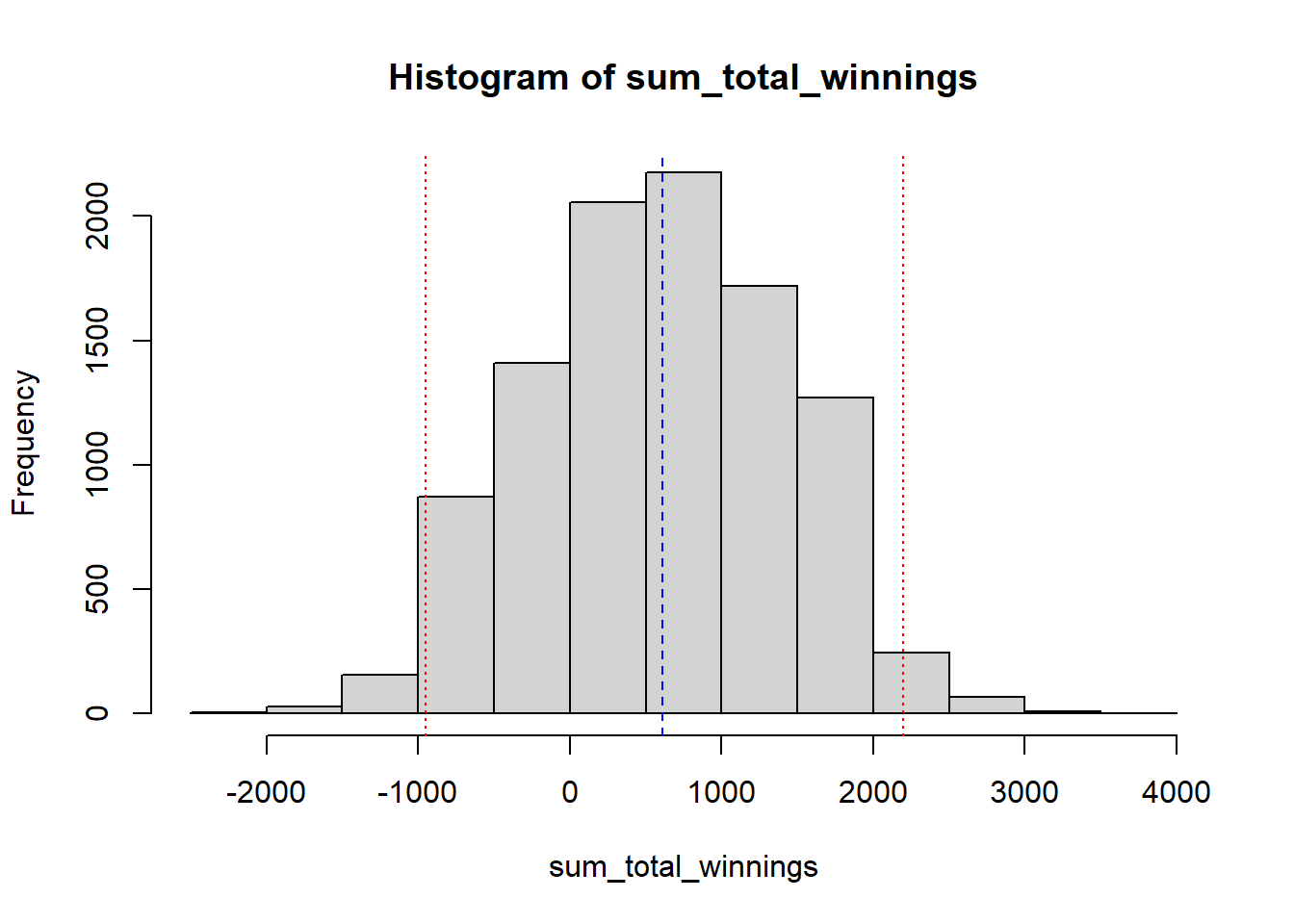
11.1.2 Value-at-risk
Think of value at risk as a probability value. In our case, we would like to understand what the probability of incurring a loss in this game is.
To find the probability of getting 0 or less in the sum_total_winnings vector, you can use the mean() function in R to calculate the proportion of values in the vector that are 0 or less. Here is an example of how you could do this:
# Calculate the proportion of values in the sum_total_winnings vector that are 0 or less
value_at_risk <- mean(sum_total_winnings <= 0)

print(value_at_risk)
#> [1] 0.2464
Its seems like there is 24.64% likely to incur 0 or loss. We can show it graphically in the histogram as:
# Plot a histogram of the sum_total_winnings vector
hist(sum_total_winnings, col = "steelblue")

# Add lines to the histogram showing value 0
abline(v = 0, col = "red", lty = 3, lwd = 2)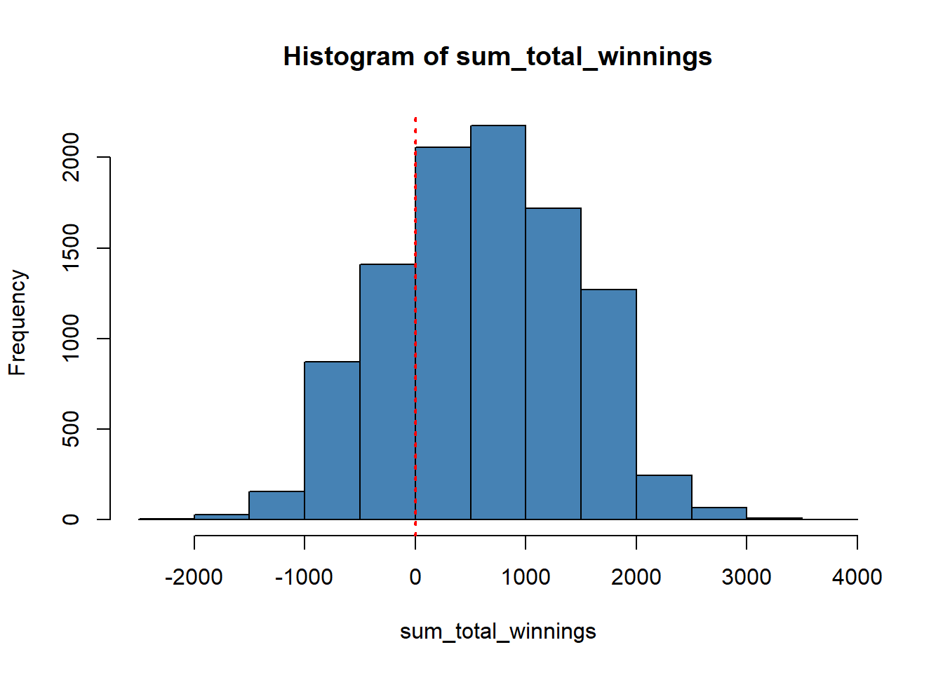
11.2 Measure of dispersion
So far, we have been discussing central tendencies like mean and median. We quickly looked into the dispersion of data with 2.5% and 97.5% quantiles. Let’s examine a few more measures of dispersion.
- The mean deviation is a measure of dispersion in a dataset. It is calculated as the average absolute difference between the dataset’s values and the dataset’s mean. For example, let’s say data is \(x\) and the mean of data is \(\bar{x}\). Then deviation can be defined as \(x - \bar{x}\).
# Define a dataset containing the values 1, 2, 3, 4, 5
dataset <- c(1, 2, 3, 4, 5)

# Calculate the mean of the dataset
mean_value <- mean(dataset)

# Calculate the deviation of the dataset
deviation_value <- dataset - mean_value

# print the deviation
print(deviation_value)
#> [1] -2 -1  0  1  2
Here is one statistical property. The sums of these deviations \(\sum (x-\bar{x})\) is always zero and also the means of deviation \(\frac{\sum (x-\bar{x})}{n}\) is zero. Lets verify that.
# Sum of deviations
sum(deviation_value)
#> [1] 0

# Sum of deviations
mean(deviation_value)
#> [1] 0
Variance: Variance is another measure of dispersion in a dataset. It is calculated as the average squared difference between the dataset’s values and the dataset’s mean. As you saw, the mean of deviations is zero, so it’s tricky to interpret 0. So, another approach is to square the deviation and take the mean as \(var = \frac{\sum (x-\bar{x})^2}{n}\). However, the issue is the unit of variance. It squares the unit. If your data is in the dollar, the unit of variance is unit squared. Again it creates slight trouble to interpret. One way to solve the issue is to take the square root.
Standard deviation: Standard deviation is a measure of dispersion in a dataset. It is calculated as the square root of the variance of the dataset as \(\sigma = \sqrt \frac{\sum (x-\bar{x})^2}{n}\).
11.3 Z-scores
We will focus little more into the standard deviation. As the name suggests standard deviation allows to standardize the data. The z-score, also known as the standard score, is a measure of how many standard deviations a value is from the mean of a dataset. It is calculated by subtracting the mean of the dataset from the value, and dividing the result by the standard deviation of the dataset.
The standardized data is called as z-scores, which can be written as \(Z=\frac{x-\bar{x}}{\sigma}\). It can simply be interpreted as how many standard deviation the data is from it’s mean.
z_score_manual <- (dataset - mean(dataset))/sd(dataset)
print(z_score_manual)
#> [1] -1.2649111 -0.6324555  0.0000000  0.6324555  1.2649111
To calculate the z-score in R, you can use the scale() function. Here is an example of how you could do this:
z_score <- scale(dataset, center = mean(dataset), scale = sd(dataset))
print(z_score)
#>            [,1]
#> [1,] -1.2649111
#> [2,] -0.6324555
#> [3,]  0.0000000
#> [4,]  0.6324555
#> [5,]  1.2649111
#> attr(,"scaled:center")
#> [1] 3
#> attr(,"scaled:scale")
#> [1] 1.581139
The z-score is helpful because it allows you to compare values from different datasets by standardizing them. For example, if you have two datasets with various means and standard deviations, you can calculate the z-scores for the values in each dataset and compare them directly.
Let me show you how z-scores allow comparing two different datasets. For example, consider the following two datasets.
# Define the first dataset
dataset1 <- c(1, 2, 3, 4, 5)

mean(dataset1)
#> [1] 3
sd(dataset1)
#> [1] 1.581139

# Define the second dataset
dataset2 <- c(10, 20, 30, 40, 50)

mean(dataset2)
#> [1] 30
sd(dataset2)
#> [1] 15.81139
The mean and standard deviation of dataset1 are 3 and 1.5811388, respectively. The mean and standard deviation of dataset2 are 15.8113883 and 15.8113883, respectively. If you calculate the z-score for the value 2 in dataset1 and the value 20 in dataset2, you will get the following results:
# Calculate the z-score for the value 2 in dataset1
z_score1 <- scale(2, center = mean(dataset1), scale = sd(dataset1))
z_score1
#>            [,1]
#> [1,] -0.6324555
#> attr(,"scaled:center")
#> [1] 3
#> attr(,"scaled:scale")
#> [1] 1.581139

# Calculate the z-score for the value 20 in dataset2
z_score2 <- scale(20, center = mean(dataset2), scale = sd(dataset2))
z_score2
#>            [,1]
#> [1,] -0.6324555
#> attr(,"scaled:center")
#> [1] 30
#> attr(,"scaled:scale")
#> [1] 15.81139
This code will first calculate the mean and standard deviation of the dataset using the mean() and sd() functions. It will then calculate the z-score for the value 2 by subtracting the mean from the value and dividing the result by the standard deviation using the scale() function. The result will be stored in the z_score variable, containing the z-score for the value 2. In this example, the z_score variable will have the value -0.6324555.
Note that mean of z-scores is 0, and the standard deviation is 1. Let’s check.
11.4 Normal distribution and standard normal distribution
A normal distribution is a type of continuous probability distribution that is defined by a symmetrical bell-shaped curve. This type of distribution is commonly used in statistics to model the distribution of a continuous random variable.
A normal distribution is defined by two parameters: the mean, which is the average value of the distribution, and the standard deviation, which is a measure of the spread of the distribution. The mean and standard deviation determine the shape and location of the normal distribution curve.
A normal distribution has several important properties, including:
- The mean, median, and mode of the distribution are all equal.
- The curve is symmetrical, with the left and right halves being mirror images of each other.
- As the standard deviation increases, the curve becomes wider and flatter.
- A normal distribution is often used in statistics to model the distribution of a continuous random variable, such as the height of a population, the weight of a sample of fruits, or the time taken to complete a task. It is particularly useful because of its symmetrical shape and its mathematical properties, which allow for easy calculation of probabilities and confidence intervals.
Let’s plot the histogram of sum_total_winnings.
hist(sum_total_winnings, main = "Does it look normal to you?")
abline(v = mean(sum_total_winnings), col = "red", lty = 9)
abline(v = median(sum_total_winnings), col = "blue", lty = 2)
The mean and median are about the same. The curve looks symmetrical, too, so it is normal. We do have statistical tests to verify the normal distribution. We will explore those later in our class.
If we divide the data by its standard deviation, we get z-scores, defined as the standard normal distribution. A standard normal distribution is a normal distribution with a mean of 0 and a standard deviation of 1. It is a special case of the normal distribution and is often used in statistics as a reference distribution to compare other normal distributions.
The following probability density function defines the standard normal distribution:
\[ f(x) = \frac{1}{\sqrt{2\pi}}e^{-\frac{x^2}{2}} \]
This function describes the probability density at any given value of x, which is the height of the normal distribution curve at that value. As you can see, the standard normal distribution has a mean of 0 and a standard deviation of 1.
A standard normal distribution has several important properties, including:
- The total area under the curve is equal to 1, which represents the total probability of all possible outcomes.
- The curve is symmetrical, with the left and right halves being mirror images of each other.
- The mean, median, and mode of the distribution are all equal to 0.
- The curve is always the same shape, regardless of the value of the standard deviation.
- A standard normal distribution is often used as a reference distribution to compare other normal distributions to. It is particularly useful because of its symmetrical shape and its mathematical properties, which allow for easy calculation of probabilities and confidence intervals.
Let’s plot the histogram of z-scores of sum_total_winnings.
z_score_wininigs <- scale(sum_total_winnings, center = mean(sum_total_winnings), scale = sd(sum_total_winnings))
hist(z_score_wininigs, main = "Does it look standard normal to you?")
abline(v = mean(z_score_wininigs), col = "red", lty = 9)
abline(v = median(z_score_wininigs), col = "blue", lty = 2)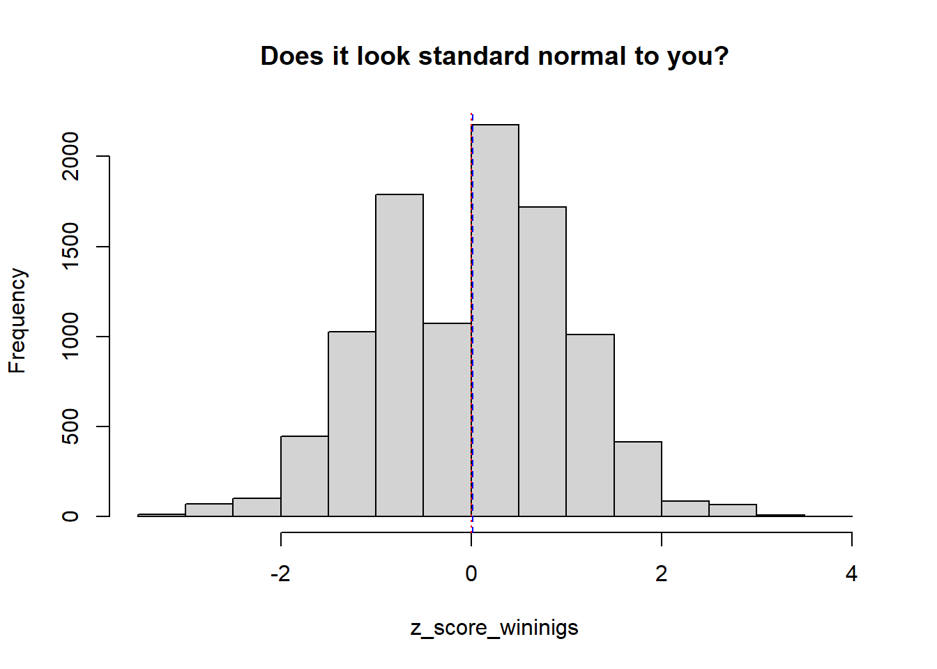
We might see some breaks here. This is because our day trading was a discrete problem, not a continuous one. Visually, the mean, median, and mode are centered at zero and symmetrical, so it seems standard normal. We can not exploit the properties of the standard normal curve. Let’s check the critical values.
11.5 Critical values
The critical values of Z are the values that are used to determine the confidence interval of a population mean in a normal distribution. The confidence interval is the range of values within which the population mean is likely to fall, given a certain confidence level.
For a normal distribution, the critical values of Z for a 90% confidence interval are -1.645 and 1.645. For a 95% confidence interval, they are -1.96 and 1.96, and for a 99% confidence interval, they are -2.575 and 2.575.
How are these critical values generated? Here is a quick intuition. First, let’s reprint the sum_total_winnings and z_score_wininigs 90%, 95%, and 99% quantiles. Then, take a closer look at the z_score_wininigs’ quantiles. Those intervals look similar to the critical values.
# Use the quantile() function to compute the quantiles for sum_total_winnings
quantile(sum_total_winnings, probs = c(0.005, 0.025, 0.05, 0.95, 0.975, 0.995))
#>  0.5%  2.5%    5%   95% 97.5% 99.5%
#> -1400  -950  -725  1975  2200  2650

# Use the quantile() function to compute the quantiles for z_score_wininigs
quantile(z_score_wininigs, probs = c(0.005, 0.025, 0.05, 0.95, 0.975, 0.995))
#>      0.5%      2.5%        5%       95%     97.5%     99.5%
#> -2.516156 -1.953012 -1.671440  1.707424  1.988996  2.552140
11.6 Hypothesis testing with z-score
Hypothesis testing is a statistical procedure used to determine whether there is sufficient evidence in a sample of data to infer a certain relationship or difference between two or more population characteristics. In hypothesis testing, a researcher first states a hypothesis. The hypothesis may be based on previous research or existing theories, or it may be a new idea that the researcher wants to test. Next, the researcher collects a sample of data and uses statistical tests to evaluate the strength of the evidence in the sample in support of the hypothesis. If the evidence is strong enough, the researcher can reject the null hypothesis and conclude that the alternative hypothesis is true. Hypothesis testing is an important tool in statistical analysis, as it allows researchers to draw conclusions about population characteristics based on sample data. By testing hypotheses, researchers can gain insight into the relationships between variables and make informed decisions based on the evidence.
In our case, we would like to test the hypothesis that the average of winnings is zero. One way is to look into the 95% confidence interval quickly. The 95% confidence interval of the winnings is:
Then check if the zero exists between the lower bound -950 and upper bound 2200 or not. If zero exits, your average of winnings is likely zero. Unfortunately, that’s our case.
Alternatively, we can formally test it with z-scores of 0 in the sum_total_winnings. The idea is to ask how much standard deviation zero is away from the mean of sum_total_winnings.
\[Z = \frac{0-\bar{x}}{\sigma}\]
If we examine the zscore_0, its value is -0.764152, which ranges between the 95% critical value of -1.96 and 1.96. This suggests that the average of winnings can be zero.