Lecture 15 Gradient descent for simple regression
15.1 Scatter plot
A scatter plot is a data visualization type showing the relationship between two variables. It is called a scatter plot because it uses dots or markers to represent the data points, which are plotted on a two-dimensional grid with the values of one variable on the horizontal axis and the values of the other variable on the vertical axis.
Scatter plots are helpful in visualizing the relationship between two variables because they allow us to see the data points and how they are distributed. For example, if there is a strong linear relationship between the two variables, we might see a clear pattern in the data points that forms a straight line on the scatter plot. On the other hand, if there is no relationship or a more complex relationship between the variables, the data points might be more scattered and not form a clear pattern.
Scatter plots are also helpful in identifying trends and outliers in the data. For example, if there is a trend in the data where one variable increases as the other variable increases, we might see a cluster of data points that forms a diagonal line on the scatter plot. On the other hand, outliers are data points that are significantly different from the rest of the data and might be indicated by dots that are far away from the main cluster of data points.
In general, scatter plots help explore and visualize the relationship between two variables in a dataset. They can help us understand the data and identify patterns and trends that might not be apparent from the raw data.
Let me generate some data and plot them in R.
# Generate some dummy data
x <- c(1, 2, 3, 4, 5)
y <- c(3, 4, 8, 12, 11)
plot(x = x, y = y, main = "Scatter plot", xlim = c(-2, 7), ylim = c(0, 16), col = "black")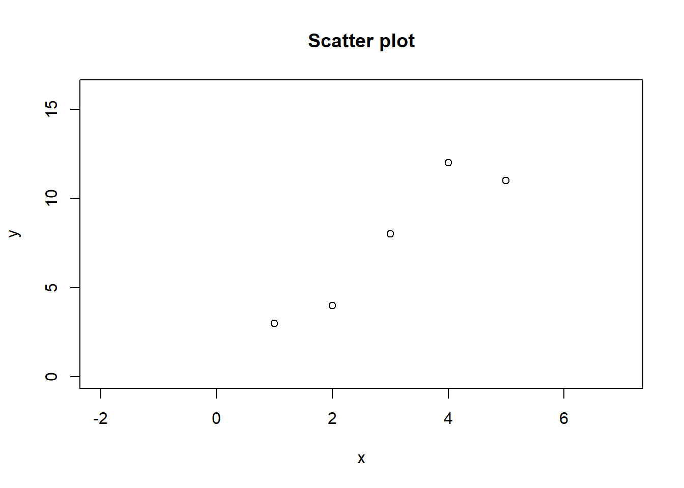
This code creates a scatter plot using the plot function in R. The plot function takes several arguments that specify the plotted data, the plot’s appearance, and other options.
The first two arguments to the plot function are x and y, which specify the data to be plotted. The x and y values are defined as vectors using the c function in this case. The x vector contains the values 1, 2, 3, 4, and 5, and the y vector contains the values 3, 4, 8, 12, and 11. These values will be used to create the scatter plot, with the values in the x vector plotted on the horizontal axis and the values in the y vector plotted on the vertical axis.
The plot function also takes the main argument, which specifies the plot’s title. In this case, the title is set to “Scatter plot”. Finally, the xlim and ylim arguments specify the range of values to be shown on the horizontal and vertical axes, respectively. In this case, the range of values for the horizontal axis is set from -2 to 7, and the range for the vertical axis is set from 0 to 16.
The col argument specifies the color of the data points on the scatter plot. In this case, the color is set to “black”.
15.2 Intuition of simple linear regression
What kind of trend do you see in these data? It’s tough to miss- a positive upward trend.
Now, use a scale ruler and pen to draw a straight line on this scatter plot that you think is the best. You will probably draw something like this.
plot(x = x, y = y, main = "Scatter plot", xlim = c(-2, 7), ylim = c(0, 16), col = "black")
abline(lm(y~x), col="red", lwd=2, lty = 3)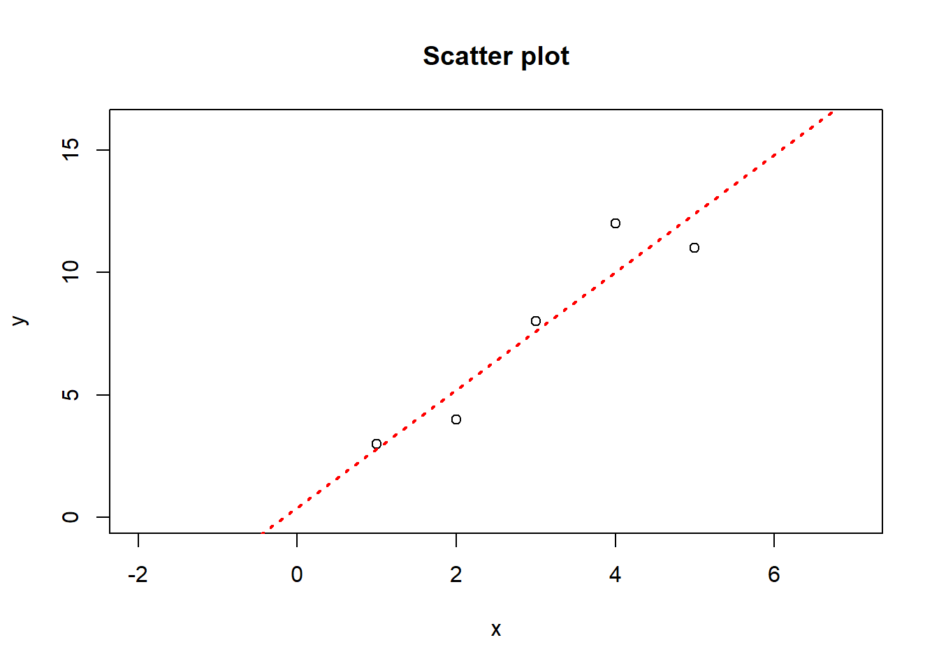
That’s what we will do in simple linear regression. We will find the best fit line between the two variables. When we say a simple linear regression, it can be expressed with an equation of straight line as \[y = mx + c\]
However, we will write this as \[y = \beta_0 + \beta_1x\]
where slope \(m = \beta_1\) and y-intercept \(c = \beta_0\). You may think economists tend to use Greek letters to look cool. However, we use Greek letters whenever we feel the quantity can be estimated with enough data.
When we say estimate– we mean the best guess or best prediction of the value of \(y\) with the best guess of true \(\beta_0\) as \(\widehat{\beta_0}\) and \(\beta_1\) as \(\widehat{\beta_1}\).
Thus we can express as: \[\widehat{y} = \widehat{\beta_0} = \widehat{\beta_1}x\]
Therefore there will be some residual between actual \(y\) and \(\widehat{y}\). \[e = y - \widehat{y}\]
For the sake of our example, let’s say initialize (best guess) the value of \(\widehat{\beta_0}\) and \(\widehat{\beta_1}\) as 1 and 2. Then, for each value of x given previously as 1, 2, 3, 4, and 5, the corresponding predicted \(y\) or \(\widehat{y}\) would be 3,5,7,9 and 11.
| x | y | \(\widehat{y}\) when \(\widehat{\beta_0}\) = 1 & \(\widehat{\beta_1}\) = 2 | \(e = y - \widehat{y}\) | e^2 |
|---|---|---|---|---|
| 1 | 3 | 3 | 0 | 0 |
| 2 | 4 | 5 | -1 | 1 |
| 3 | 8 | 7 | 1 | 1 |
| 4 | 12 | 9 | 3 | 9 |
| 5 | 11 | 11 | 0 | 0 |
The difference between actual \(y\) and predicted \(\widehat{y}\) is residuals or error \(e = y - \widehat{y}\) is given as 0,-1,1,3, and 0.
In a regression analysis, the residuals represent the difference between the observed and predicted values. Therefore the sum or the mean of the residuals is not always zero. The sum or the mean of the residuals will be zero only if the predicted values perfectly match the observed values. However, this is often not the case, especially when there is noise or other sources of error in the data.
Now we want to optimize the error. One way to do this is to square the residual and take a mean or mean squared error given as \[MSE = \frac{\sum e^2}{n}=n^{-1}\sum e^2 = n^{-1}\sum(y-\widehat{y})^2\].
In another word, we would like to find \(\widehat{\beta_0}\) and \(\widehat{\beta}\) that minimizes \(MSE\).
Analytically, we have to take the derivative or gradient of \(MSE\) w.r.t \(\widehat{\beta_0}\) and \(\widehat{\beta}\), then set them to zero and solve it.
\[\frac{\partial n^{-1}\sum e^2}{\partial \widehat{\beta_0}}=\frac{\partial n^{-1}\sum(y-\widehat{y})^2}{\partial \widehat{\beta_0}}= \frac{n^{-1}\partial \sum(y-\widehat{y})^2}{\partial (y-\widehat{y})} \frac{\partial (y-\widehat{y})}{\widehat{\beta_0}}=2n^{-1}\sum(y-\widehat{y})\frac{\partial (y-\widehat{\beta_0}-\widehat{\beta_1}x)}{\widehat{\beta_0}}=-2n^{-1}\sum(y-\widehat{y})\] \[\frac{\partial n^{-1}\sum e^2}{\partial \widehat{\beta_0}}=-2n^{-1}\sum(y-\widehat{y})=-2\frac{\sum e}{n}\]
Similarly,
\[\frac{\partial n^{-1}\sum e^2}{\partial \widehat{\beta_1}}=-2n^{-1}\sum(y-\widehat{y})=-2\frac{\sum ex}{n}\]
Now let’s use gradient descent using R.
To begin let’s first initialize \(\widehat{\beta_0}\) and \(\widehat{\beta}\) as zero, we can choose any numbers. Also set the learning rate as 0.1.
# Generate some dummy data
x <- c(1, 2, 3, 4, 5)
y <- c(3, 4, 8, 12, 11)

# Set the learning rate
alpha <- 0.01

# Set the initial values of the coefficients
beta0 <- 0
beta1 <- 0
Let’s use the gradient descent on \(\widehat{\beta_0}\) and \(\widehat{\beta}\) to minimize the \(MSE\), let’s call it the cost.
results <- list()
# Define the gradient descent algorithm
for (i in 1:10000) {
  # Compute the predicted values
  y_pred <- beta0 + beta1 * x

  # Compute the errors
  # computer scientists tend to use error = y_pred - y, but we will remain consistent with economist
  # taking square error of (y_pred - y) seem same as (y - y_pred), but there are some fundamental issues
  error <- y - y_pred

  # Compute the cost
  cost <- mean((error^2))

  # Update the coefficients
  # Since computer scientist do y_pred-y, their gradient would be 2*mean(error)
  beta0 <- beta0 - alpha * (-2)*mean(error)

  #Since computer scientist do y_pred-y, their gradient would be 2*mean(error * x)
  beta1 <- beta1 - alpha * (-2)*mean(error * x) #

  results[[i]] <- data.frame("iteration" = i,"beta0" = beta0, "beta1" = beta1, "MSE" = cost)

  # The alpha * (-2)*mean(error) mathematically means (-2 * alpha)(mean(error))
  # which actually doubles your learning rate, which is bad for precision.
  # So the value of betas can be expressed as
  # beta0 <- beta0 + alpha*mean(error)
  # beta1 <- beta1 + alpha*mean(error * x)

}
In this code, the cost function is the mean squared error between the predicted values of the dependent variable (y_pred) and the true values of the dependent variable (y). The predicted values are computed using the current values of the coefficients beta0 and beta1, which are updated in each iteration of the algorithm using the gradient of the cost function with respect to the coefficients.
The gradient descent algorithm is run for 10,000 iterations, which means that the values of beta0 and beta1 are updated 10,000 times in order to find the values that minimize the cost function. The learning rate alpha determines the size of the updates to the coefficients in each iteration and is a hyperparameter that needs to be set before running the algorithm.
We need to make a few adjustments to this algorithm in which we allow the algorithm to stop after it reaches the convergence or a certain threshold. Second, we keep the learning parameter as per our wish and not twice the size.
# Generate some dummy data
x <- c(1, 2, 3, 4, 5)
y <- c(3, 4, 8, 12, 11)

# Set the learning rate
alpha <- 0.01

# Set the initial values of the coefficients
beta0 <- 0
beta1 <- 0

# Set the convergence threshold
convergence_threshold <- 1e-10

# Set the initial value of the previous cost
prev_cost <- Inf

# Initialize the iteration counter
iteration <- 0

# Start the loop
while (TRUE) {
  # Increment the iteration counter
  iteration <- iteration + 1

  # Compute the predicted values
  y_pred <- beta0 + beta1 * x

  # Compute the errors
  error <- y - y_pred

  # Compute the cost
  cost <- mean((error^2))

  # Print the current state
  # print(paste(iteration, beta0, beta1, cost, sep = ", "))

  # Store the results
  results <- data.frame("iteration" = iteration,"beta0" = beta0, "beta1" = beta1, "MSE" = cost)

  # Check for convergence
  if (abs(cost - prev_cost) < convergence_threshold) {
    break
  }

  # Update the previous cost
  prev_cost <- cost

  # Update the coefficients
  beta0 <- beta0 - alpha * (-1)*mean(error)
  beta1 <- beta1 - alpha * (-1)*mean(error * x)
}
The code uses the gradient descent algorithm to fit a simple linear regression model into a dummy data set. The data consists of 5 pairs of values (x and y), and the goal is to find the values of the coefficients beta0 and beta1 that best fit the data.
The gradient descent algorithm works by starting with initial values for the coefficients (in this case, beta0 = 0 and beta1 = 0) and then iteratively updating the values of the coefficients in a way that reduces the cost (which is a measure of how well the model fits the data). The cost is computed using the mean squared error (MSE) between the predicted values and the actual values of y.
At each iteration, the code computes the predicted values of y, the errors, and the cost. It then updates the coefficients by moving in the opposite direction of the gradient (which is the derivative of the cost with respect to the coefficients). This update is scaled by the learning rate, which determines the size of the step taken in the opposite direction of the gradient.
The code includes a convergence check that compares the current cost with the previous cost and terminates the loop if the difference is less than the convergence threshold (which is set to 1e-5 in this example). This ensures that the algorithm will continue running for a while but will stop when it reaches a point where further updates to the coefficients will not likely improve the model significantly.
Let’s examine the results of the algorithm to the analytic solution.
results
#>   iteration     beta0    beta1  MSE
#> 1      3793 0.4004022 2.399889 1.52
summary(lm(y~x))
#>
#> Call:
#> lm(formula = y ~ x)
#>
#> Residuals:
#>    1    2    3    4    5
#>  0.2 -1.2  0.4  2.0 -1.4
#>
#> Coefficients:
#>             Estimate Std. Error t value Pr(>|t|)
#> (Intercept)   0.4000     1.6693   0.240   0.8261
#> x             2.4000     0.5033   4.768   0.0175 *
#> ---
#> Signif. codes:
#> 0 '***' 0.001 '**' 0.01 '*' 0.05 '.' 0.1 ' ' 1
#>
#> Residual standard error: 1.592 on 3 degrees of freedom
#> Multiple R-squared:  0.8834, Adjusted R-squared:  0.8446
#> F-statistic: 22.74 on 1 and 3 DF,  p-value: 0.01752
The summary() function in R is used to generate a summary of a model. In this case, the lm() function is used to fit a linear regression model to the data, with y as the response variable and x as the predictor variable. The summary() function is then applied to the resulting model object to generate a summary of the model fit.
The summary of a linear regression model typically includes information such as the coefficients (i.e., the estimated values of beta0 and beta1 in this case), the intercept, the residuals (i.e., the difference between the observed values of y and the predicted values), the R-squared value (which indicates how well the model fits the data), and the F-statistic (which is used to assess the overall significance of the model). The summary can also include other diagnostic information, such as the distribution of the residuals, which can be useful for checking the assumptions of the model.
But when we compare the results, it seems we were pretty close!
15.3 Exercise
E1. Use the following data and estimate the coefficients.
n <- 1000
x <- rnorm(n)
y <- 1 - 4 * x + rnorm(n)
# you can see the actual estimate of intercept and slope with
# summary(lm(y~x))
# Use gradient descent approach to identify those coefficients.
E2. Use the following data and estimate the coefficients.