Lecture 4 For loop and probability
4.1 For loop control flow statement
A for loop is a control flow statement in programming that allows a set of instructions or operations to be repeated a specified number of times, or until a certain condition is met. For loops are a common feature of many programming languages, including R, and they are often used to perform repetitive operations on a set of data or to iterate over the elements of a data structure.
A for loop typically has three components: an initial value, a condition, and an update expression.
The initial value is the starting point for the loop, and it is typically defined as a variable that will be used to store the current value of the loop.
The condition is a logical expression that is evaluated at the start of each iteration of the loop, and it determines whether the loop should continue or stop.
The update expression is a statement that is executed at the end of each iteration of the loop, and it updates the value of the loop variable in order to move the loop to the next iteration.
4.2 Probability of heads
Let me ask a very mundane question. What is the probability of getting heads when flipping a fair coin?
The probability of getting heads when flipping a coin is 1/2, or 0.5. This is because a coin has two possible outcomes (heads or tails), and each outcome has an equal probability of occurring. When flipping a fair coin, there is a 50% chance of it landing on heads and a 50% chance of it landing on tails. Therefore, the probability of getting heads is 1/2, or 0.5.
But is there a way to verify with experimentation?
One way to verify the probability of getting heads when flipping a coin is to experiment. To do this, you would need to flip a coin a large number of times (e.g., 100, 1000, or more) and keep track of the number of times it lands on heads. After flipping the coin a sufficient number of times, you can calculate the percentage of times it landed on heads. This should be close to the expected probability of 1/2, or 0.5. If the experimental result is significantly different from the expected probability, it may indicate that the coin is not fair and is biased towards one side or the other.
4.3 Experimenting with 100 coin flips
To simulate a coin flip 100 times and store the values, you can use a for loop in R to iterate over the flips and store the results in a vector. Here is an example of how to do this:
# create a vector of the values "head" and "tail"
coin_flip <- c("head", "tail")

# create an empty vector to store the results
results <- vector()

# simulate the coin flips
for (i in 1:100) {
  # shuffle the values in the vector
  coin_flip <- sample(coin_flip)

  # store the first value in the shuffled vector
  results[i] <- coin_flip[1]
}

# print the results vector
print(results)
#>   [1] "head" "tail" "head" "head" "head" "head" "head"
#>   [8] "head" "tail" "head" "head" "head" "head" "tail"
#>  [15] "tail" "head" "tail" "tail" "head" "head" "head"
#>  [22] "head" "head" "tail" "tail" "head" "tail" "head"
#>  [29] "head" "head" "tail" "tail" "head" "tail" "tail"
#>  [36] "tail" "tail" "head" "tail" "head" "tail" "head"
#>  [43] "head" "head" "tail" "head" "tail" "tail" "tail"
#>  [50] "head" "head" "head" "head" "head" "head" "head"
#>  [57] "head" "tail" "tail" "tail" "tail" "head" "tail"
#>  [64] "tail" "head" "head" "head" "head" "head" "tail"
#>  [71] "head" "head" "head" "tail" "head" "head" "tail"
#>  [78] "tail" "tail" "head" "tail" "head" "head" "tail"
#>  [85] "tail" "head" "head" "head" "head" "tail" "tail"
#>  [92] "head" "tail" "tail" "tail" "head" "head" "tail"
#>  [99] "head" "tail"
In this code, we first create a vector called coin_flip that holds the values “head” and “tail”. We then create an empty vector called results to store the outcomes of the coin flips. Next, we use a for loop to simulate 100 coin flips, by using the sample() function to shuffle the values in coin_flip and then storing the first value in the shuffled vector in the results vector. Finally, after the for loop has been completed, we print the results vector to the R console to see the outcomes of the simulated coin flips.
Note that the result of this simulation will vary each time it is run, due to the random nature of the sample() function. However, the results vector will always contain 100 elements, each of which will be either “head” or “tail”. You can use this technique to simulate any random event that involves a set of possible outcomes and store the results for further analysis.
To count the number of “head” outcomes from the results of a coin flip simulation, you can use the sum() function in R to count the number of times the value “head” appears in the results vector.
# count the number of "head" outcomes in the results vector
head_count <- sum(results == "head")

# print the number of "head" outcomes
print(head_count)
#> [1] 58
We use the sum() function to count the number of times the value “head” appears in the results vector and assign this value to the head_count variable. Finally, we print the head_count variable to the R console to see the number of “head” outcomes from the simulated coin flips.
The probability of getting “head” when flipping a fair coin is 50%, because a fair coin has an equal chance of landing on either “head” or “tail” when flipped. This means that if you flip a fair coin 100 times, you can expect to get approximately 50 “head” outcomes and 50 “tail” outcomes, although the exact number of each outcome may vary slightly due to randomness.
From the above example, the probability of getting head is:
Given these 100 trials, we got 58 heads. Hence the probability of getting head is 0.58, which is close to a theoretical value of probability \(\frac{1}{2}=0.5\).
If you have not found the exact 50% probability, you can increase the experimentation trails to say 10000 times.
# create an empty vector to store the results
results <- vector()
# simulate the coin flips
for (i in 1:10000) {
  results[i] <- sample(x = c("head", "tail"), size = 1, replace = T)
}

head_prob <-  sum(results == "head") / length(results)

head_prob
#> [1] 0.4976
Actually there is a faster and better way to do it by simply changing the size in the sample() arguments.
# This doesn't need for loop
results <- sample(x = c("head", "tail"), size = 10000, replace = T)

head_prob <-  sum(results == "head") / length(results)

head_prob
#> [1] 0.4978
As you see that if you increase the experimentation the probability of getting head converges to zero. Let me show you one more simulation, where I will do the experiments and record the probability of getting head and plot it.
R <- seq(from = 1, to = 10000, by = 100)
head_prob <- vector()
# simulate the coin flips
for (i in 1:length(R)) {
  results <- sample(x = c("head", "tail"), size = R[i], replace = T)
  head_prob[i] <-  sum(results == "head") / length(results)
}
The first line of code creates a sequence of numbers from 1 to 10000 in increments of 100, and assigns this sequence to the variable R. The next line creates an empty vector called head_prob, which will be used to store the probability of flipping a head for each iteration of the experiment.
The for loop then iterates over the sequence stored in R. For each value of R, the code uses the sample function to simulate flipping a coin R[i] times. This function returns a vector of R[i] elements, each of which is either “head” or “tail”. The results variable is assigned this vector.
Next, the code uses the sum function to count the number of elements in results that are equal to “head”, and divides this number by the total number of elements in results to calculate the probability of flipping a head. This probability is then stored in the ith element of the head_prob vector.
After the for loop is finished, the head_prob vector will contain the probability of flipping a head for each value of R. This can then be used to visualize the relationship between the number of coin flips and the probability of flipping a head.
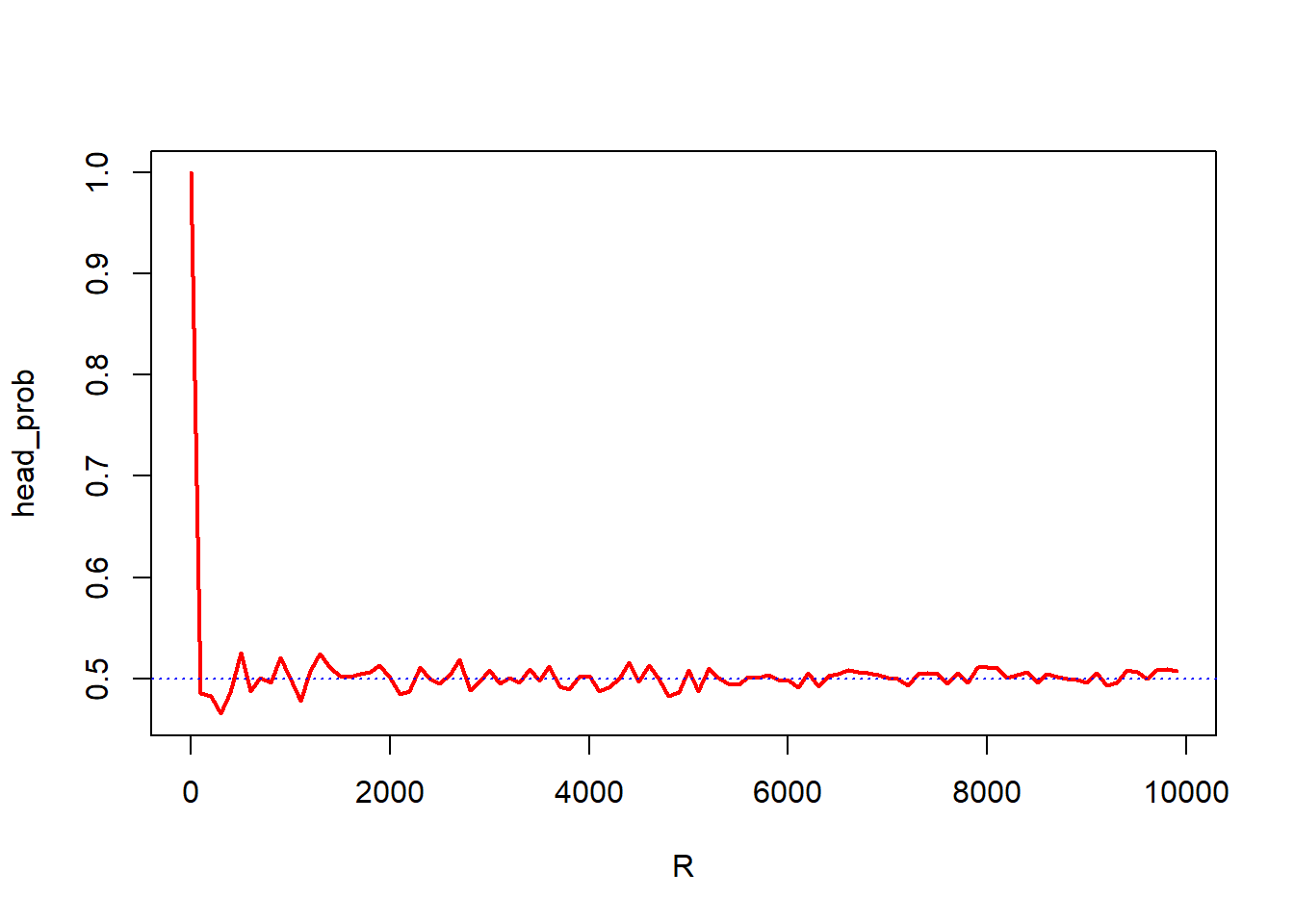
This code is plotting the results of the coin flip experiment in R. The plot function is used to create a line plot with the x-axis representing the number of coin flips (stored in the R variable), and the y-axis representing the probability of flipping a head (stored in the head_prob variable). The type = “l” argument tells the function to create a line plot, and the col = “red” and lwd = 2 arguments specify the color and thickness of the line, respectively.
The abline function is then used to add a horizontal line to the plot at the y-value of 0.5. This line represents the expected probability of flipping a head if the coin is fair. The h = 0.5 argument specifies the y-value of the line, the lty = 3 argument specifies the line type (in this case, a dotted line), and the col = “blue” argument specifies the color of the line.
Together, these two lines of code create a line plot that shows the relationship between the number of coin flips and the probability of flipping a head. The horizontal line at 0.5 serves as a reference point to show whether the coin is fair or not. If the line representing the probability of flipping a head is above the 0.5 line, it indicates that the coin is biased towards flipping heads. If it is below the 0.5 line, it indicates that the coin is biased towards flipping tails.
4.4 Exercises
E1. Suppose you roll a standard six-sided die 10000 times. What is the probability of getting a 6 on any given roll, and how many times can you expect to get a 6 in the 10000 rolls? Show the solution with R codes.
E2. Suppose you roll two standard six-sided dice and sum the outcomes. What is the probability of getting each possible sum, and which sum has the highest probability? Show the solution with R codes.
E3. Suppose you draw 7 cards from a deck of 52 standard playing cards with and without replacement. What is the expected distribution of the sums of the 7 cards? Show the solution with R codes.
Hint: To answer this question, you should first recognize that there are 13 possible values for each card, from 2 to 10, and then J, Q, K, and A. Lets call A as 1, J, Q, and, K as 11, 12, and 13 respectively. They should then calculate the probability of getting each possible sum of the 7 cards by using the formula for the probability of an event occurring: probability = number of ways the event can happen / total number of possible outcomes. Show the solution with R codes.